Give the gift of life-changing education! Donate Now!
Random Variables
A random variable must take a numerical value:
Examples: the number on a single throw of a die the height of a person
the number of cars travelling past a fixed point in a certain time But not the colour of hair as this is not a number
Continuous and discrete random variables
Continuous random variables
A continuous random variable is one which can take any value in a certain interval;
Examples: height, time, weight.
Discrete random variables
A discrete random variable can only take certain values in an interval
Examples:
Score on die (1, 2, 3, 4, 5, 6)
Number of coins in pocket (0, 1, 2, …)
Probability distributions
A probability distribution (or table) is the set of possible outcomes together with their probabilities, similar to a frequency distribution (or table).
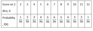
is the probability distribution (table) for the random variable, X, the total score on two dice.
Note that the sum of the probabilities must be 1 , i.e \(\sum_(x = 2)^{12}\)P(X = x ) = 1
Cumulative probability distribution
Just like cumulative frequencies, the cumulative probability, F, that the total score on two dice is less than or equal to 4 is
F(4) = P(X ≤ 4) = P(X = 2,3,4) = \(\frac{1}{36}\) + \(\frac{2}{36}\) + \(\frac{3}{36}\) = \(\frac{1}{6}\)
Note that F (4.3) means P(X ≤ 4.3) and seeing as there are no scores between 4 and 4.3 this is the same as P(X ≤ 4) = F (4)
You are expected to recognise that capital F(X)means the cumulative probability
Expectation or expected values
Expected mean or expected value of X.
For a discrete probability distribution the expected mean of X , or the expected value of X is
µ = E[X] =∑ pi xi
Expected value of a function
The expected value of any function, h(X), is defined as
E[X] = ∑ h( xi )pi
Note that for any constant, k, E[k] = k,
since ∑ kpi = k ∑pi = k × 1 = k
Expected variance
The expected variance of X is
σ2 = Var[X] = E[(X-μ)2 ] = E[X2 ] – μ2 = E[X2 ] – (E(X))2
Expectation algebra
E[aX + b] = = aE[X] + b
since ∑ xi pi = μ , and ∑ pi = 1
Var[aX + b] = E[(aX + b)2 ] – (E[(aX + b)])2
= E[(a2 X 2 + 2abX + b2 )]) – (aE[X] + b)2
= {a2 E[X 2 ] + 2ab E[X] + E[b2]} – {a2 (E[X])2 + 2ab E[X] + b2}
= a2 E[X 2 ] – a2 (E[X])2 = a2{E[X 2 ] – (E[X])2 } = a2 Var[X]
Thus we have two important results:
E[aX + b] = aE[X] + b
And Var[aX + b] = a2 Var[X] which are equivalent to the results for coding .