Give the gift of life-changing education! Donate Now!
7.1-DISCRETE PROBABILITY DISTRIBUTIONS
Discrete Random Variables
Random Variable : – represents in number form the possible outcomes, which could occur for some random experiment. Random variables which have a finite number of assigned values are called DISCRETE
Random Variables : A discrete random variable X has a set of distinct possible DISCRETE values.
X= 0, 1 , 2 , 3 , 4 , ……..
For Example:
The number of houses in your neighborhood which have a ‘power safety switch’
The number of new bicycles sold each year by a bicycle store .
The the number of defective light bulbs in the purchase order of a city store.
A Continuous Random Variable X has all possible values in some interval (on a number line.
For Example:
The heights of men could all lie in the interval 50.< x < 250 cm
The volume of water in a rainwater tank during a given month.
NOTE: A discrete random variable involves a count whereas a continuous random variable involves measurement.
Discrete Probability Distributions
Probability Distributions the set of possible values of a random variable along with the corresponding probabilities. For each random variable there is a probability distribution.
The probability· distribution of a discreet random Variable can be given :
• in table form
in graphical form
in functional form as a probability mass function P(r).
It provides us with all possible value of the variable and the probability of the occurrence of each value.
Expectation : Once a probability distribution has been explicitly defined, then this mathematical model of the experiment can be used to further analyze the experiment. One very useful piece of information that may be obtained is the expected value. The EXPECTED VALUE is that quantity that you can expect to obtain when the experiment is performed.
If there are n trials of an experiment and an event has probability p of occurring in each of the trials, then the number of times we expect the event to occur is np.
7.2 – BINOMIAL DISTRIBUTION
Consider an experiment for which there are two possible results: success if some event occurs, or failure if the event does not occur. If we repeat this experiment in a number of independent trials, we call it a binomial experiment. The probability of a success p must be constant for all trials. Since success and failure are complementary events, the probability of a failure is 1- p and is constant for all trials. The random variable Xis the total number of successes inn trials.
Binomial Distribution :
For a Binomial Distribution of n trials with the probability p of success on each trial, the mean (expectation) of the number of successes is:
µ = E(x) = np
7.3 – THE NORMAL DISTRIBUTION
The Normal Distribution is the most important distribution for a continuous random variable. Many naturally occurring phenomena have a distribution that is normal, or approximately normal. Some example are:
• Physical attributes of a population such as height and weight
• Crop yields
• Test scores taken from a large population.
Once a normal model has been established, we can use it to make predictions about a distribution.
Characteristics :


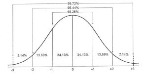
For a normal distribution with mean µ and standard deviation σ, the proportional breakdown of where the random variable could lie is given below.
Standard Normal Distribution
In a Standard Normal Distribution the mean= 0 and standard deviation= 1.
X∼N(µ,σ)
For a normal distribution other than X∼N(0,1) ,we must perform a transformation on the variables into a z-score where z =\(\frac{x-µ}{σ}\)
If each data value of a normally distributed random variable x is transformed into a z-score, the result will be the standard normal distribution.

Use the Standard Normal Table to find the cumulative area under the standard normal curve.
Inverse Normal Distribution
1.Calculating inverse normal distribution is much like calculating the normal distribution. The first thing you should do is press the ‘2ND’ button on your calculator and then press the ‘VARS’ button which has the second function (the blue text above the button) of ‘DISTR’. Once you have done this, you should see the screen shown to the right (or below if you are on a mobile device).
2. Calculating inverse normal distribution is much like calculating the normal distribution. The first thing you should do is press the ‘2ND’ button on your calculator and then press the ‘VARS’ button which has the second function (the blue text above the button) of ‘DISTR’. Once you have done this, you should see the screen shown to the right (or below if you are on a mobile device).
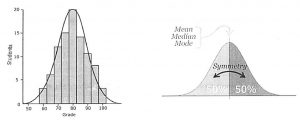
Many quantities in life are distributed symmetrically about the mean and can be described with the mathematical model known as the bell curve (normal distribution)
A population that follows the normal distribution can be described by its:
• Mean, µ, and standard deviation, σ.
• Mode= median = mean because of its symmetric shape.
• The larger the value of cr, the more dispersion of the data about the mean.
• The smaller the value of σ, the more the data cluster about the mean.
For a normal distribution, X;
 There is no easy formula for calculating areas under the normal distribution curve. Instead we approximate using z-scores, where z =\(\frac{x-µ}{σ}\). A z-score indicates the number of standard deviations a value lies from the mean. A z-score also converts a particular normal distribution to a standard normal distribution, so z-scores can be used with the areas under the normal distribution curve to find probabilities. The notation for a normal distribution is X∼N(µ,σ2). The Standard Normal Distribution is written as X∼N(0,12)) and is the distribution of z-scores of a normally distributed variable with mean = 0 and standard deviation = 1.
The process of reducing a normal distribution to the standard normal distribution X∼N(0,12) is called standardizing.
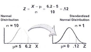
In the following example, the value x = 6.2 has been standardized to N(O, 1) using z-scores.

Recall, a negative z-score indicated that the value lies below the mean. The value also has the same position on the standard normal distribution (on the right) as the normal distribution (on the left).
Areas under the normal curve can be found on the graphing calculator using the normal(function from the DISTR menu. The syntax for this function is: normal (lower bound, upper bound, mean, standard deviation)